There is a curious phrase I keep seeing, an invocation so alien I could never imagine myself saying it.
“Follow your local covid-19 rules” it advises, ending an article on covid-19 policy, “do as your local public-health department tells you”.
Paradoxically, while covid-19 guidance varies from place to place, i.e. is “local”, a person’s reaction to these guidelines – to do as they are told – should not vary from place to place.
This strikes me as a cowardly way of trying to avoid responsibility. If you think a policy is advisable, you should advise people to follow the policy. If you think people should wear N95 masks, you should tell them to wear N95 masks, regardless of the local rules. Likewise, if you think quarantines of a certain length are not worth the cost, you should tell people to break quarantines (if they can get away with it). It’s deeply weird that someone living in place X optimally should follow one policy, and someone living in place Y – indistinguishable to X, except for different rules – should follow a different policy. Your advice isn’t gospel, what people do in the end is still their choice.
My humble request: stop pretending it is good to follow local rules. Some rules should be broken. Though if you think it takes everyone following the rules to reach salvation, you do have company.
Warning: this is a draft, but since nobody reads my blog it shouldn’t matter.
In which a group at Imperial College try to find out how many people would have died in the UK if it had policies like Sweden.
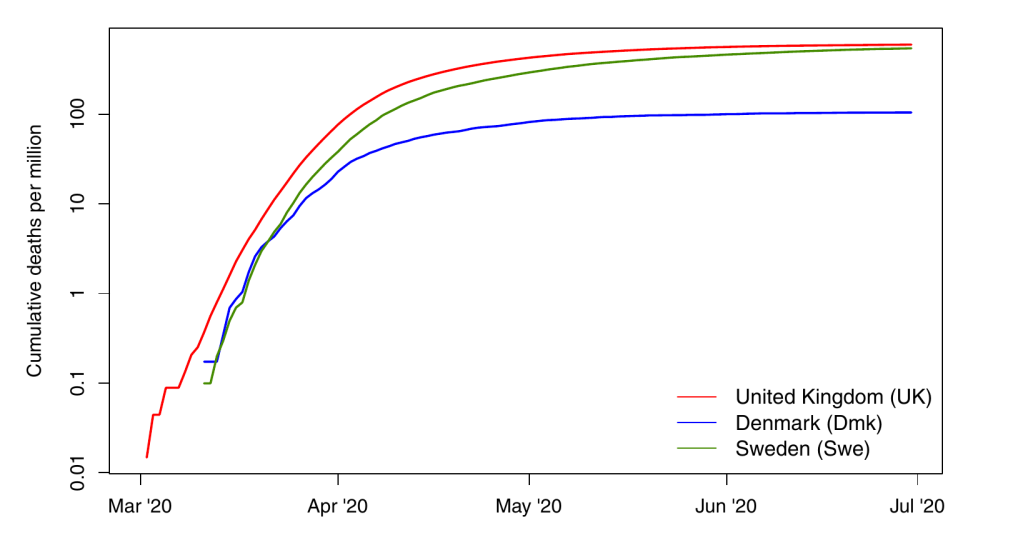
Look at the following figure illustrating cumulative covid-19 deaths in different countries, shamelessly lifted from a recent paper appearing in Nature Scientific reports1
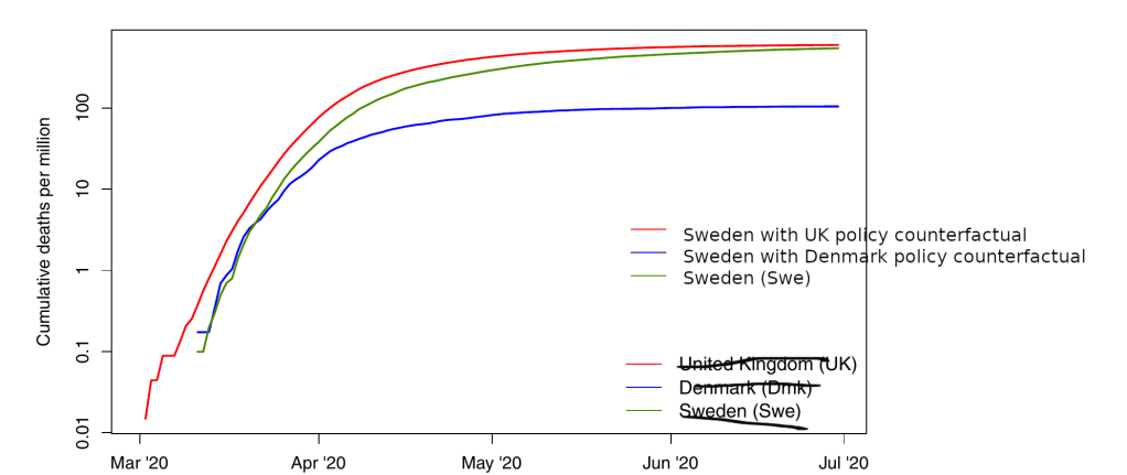
As you can see, Denmark, Sweden, and the UK had widely varying outcomes. They also had widely varying policies, so it’s natural to ask how much these are to blame. Luckily, epidemiologists have developed extremely precise tools to quantify this effect, the results of which are shown below:
The basic mathematical idea behind this approach is that obviously Sweden would have the same number of cumulative deaths as the other countries would have had if they had just used the same polices. Case closed.
This approach is used in Mishra et al., whose abstract states
We use two approaches to evaluate counterfactuals which transpose the transmission profile from onecountry onto another, in each country’s first wave from 13th March (when stringent interventions began) until 1st July 2020. UK mortality would have approximately doubled had Swedish policy been adopted, while Swedish mortality would have more than halved had Sweden adopted UK or Danish strategies.
Ok so Mishra et al. don’t actually just swap the labels, as far as I can tell they do something on the level of2 “take derivatives first, then swap labels, and then integrate again” but wrapped into the language of an SIR model. Here’s the relevant part of their paper:
If you’re not laughing/crying at the absurdity of actually publishing this kind of analysis, some more direct quotes:
We estimate that if Denmark had adopted Swedish policies, and introduced them at the same stage of its epidemic, mortality would have been between three and four (Table 1) times higher, and thus Denmark would have experienced similar per-capita mortality to Sweden
If Sweden had adopted Danish policies, both the absolute and relative approaches imply that there would have been approximately one fifth as many deaths.
The counterfactuals therefore demonstrate that small changes in the timing or effectiveness of intervention policies can lead to large changes in the resulting cumulative death toll
One fact I’ve noticed a few times from this group at Imperial College is the fact that they ascribe almost all outcomes to government policy when anybody who is following this at all should see that it isn’t even clear whether government policy is important. Thus, the article is full of the word “policy” whereas an astute reader should notice that none of the actual analysis looks at policies, it’s just comparing counts of infected/dead people, policy never actual enters the mix. This enters via phrasing like
the slightly lower effectiveness of Sweden’s policies
or
Denmark may have had marginally more effective and timely policies.
or
so that we might learn how best to control future waves, or indeed future pandemics
In fact, we might as well replace “policy” with weather everywher in the article and be no worse off for it. Or “population density”, or “trust in science” or “astrological favour”. Eventually do pay lip-service to non-policy factors also being of importance deep down in the discussion
Third, national-level Rt estimates average over a high level of geographic, social and demographic heterogeneity in transmission within each country. It is unclear how such heterogeneities between countries would determine the relative success of a country’s COVID-19 response, as opposed to differences in policy. This can be circumvented to some extent by interpreting each counterfactual scenario as an exchange of population behaviour as well as policy, although it is still true that not every country would respond in exactly the same way to each intervention.
so it all boils down to “if Sweden were the UK, it would have cases like the UK modulo initial values” which would – though not uncontroversial – be a better take than anything I’ve seen in their paper. Then again, this this was published in Nature Scientific reports, which is nice for all the grad students invovled as they now have a paper published.
Footnotes:
Not to be confused with Nature itself, twitter tells me Scieentific Reports is Nature‘s trash-basket but I have no opinion on whether or not this true apart from the fact that this particular paper belongs in the trash-basket.
Yes, I know this isn’t exactly what they do, but the analogy is pretty good though they wrap everything into a Bayesian mess.
In my last post, I proposed to improve on covid-19 IFR estimates in the literature. Mathematically, I had a rather nice model and the code would have been straightforward too.
But – I didn’t factor in how hard it would be to find raw data. So I gave up. My sincere apologies. Maybe one day someone will build a database of Covid-19 deaths on which “figuring out how many people died in age group X of country Y by date Z” is just an SQL query.
In my previous blog post, I had some comments on the statistical analysis present in some covid-19 studies. It is easy to criticize, but can I do better? Let’s find out what the data tells us about the fatality of SARS-coV-2.
Data by itself tells us nothing
Well, almost nothing – remember that we are trying to find something that should be more generally true than just for the individual data points that we have. For this we need a model, a mathematical description of the process that created the data points including the unknown parameters (in this case, the IFR) that we want to discover. It’s important to remember that such a model typically has a number of very strong assumptions, none of which are fully satisfied in real life. Some of these are simplifications, like omitting certain un-modelable complexities. Others are of a more systematic nature, such as not having access to truly random samples. It is important to remember that the conclusions reached within the model may therefore not apply to real life. This is true for any scientific study of this type. Even if the model holds exactly, there is usually some uncertainty “built in”. As shown in my previous post, scientists often don’t correctly deal with this built-in uncertainty.
Deciding on the model in advance
By tailoring a model to the data, one can strongly influence the results it shows. To avoid suspicions of this happening, and to avoid it happening inadvertently, one must always decide on the model before looking at the data. I have in fact seen some of the studies I’ll be getting data from (see previous blog post). But I have not done any statististical analysis that looks at how age/sex affects the IFR. I will use this blog post to set a fixed methodology before I look further.
Garbage in, garbage out
No matter how good you are at statistics, your conclusions can only be as good as your data. I will therefore limit myself to studies of a certain type and quality. In particular, I will only look at antibody studies in Western countries that
try to get a random sample of the whole population.
do assay validation for their tests.
come from countries not counting “suspected” covid-19 deaths like “confirmed” ones.
have age/sex statistics of the sample. I need to be able to find covid-19 death statistics as well as age statistics for the total population being sampled.
As I only have so much time, I will not look for studies not covered by the two meta-analyses in the previous blog post.
The model
I have underlined some key assumptions to show how many there are.
I start by binning ages into 10 year brackets, i.e. 0-10, 11-20, and so on, with a bin for each sex. I will label these by . For each age bracket and sex, an IFR will be estimated which I denote by . We assume that these IFR parameters are shared between studies, and do not depend on population characteristics other than age or sex.
In each study, the samples are assumed to come from some large total population (e.g. “people living in NYC”). I assume that within each age/sex bracket, the people sampled are random sample with respect to SARS-coV-2 infections. This is obviously not exactly true (for example, we can’t sample people who have already died), but seems like a reasonable approximation.
For each study, I split the total population into subpopulations per age/sex group: “has antibodies” and “does not have antibodies”. Some studies do both a PCR test and an antibody test. I do not know how to sensibly deal with this (the problem is that it’s hard to decide which date to use for death statistics if we allow for active cases), so I ignore the PCR test.
I assume that in each age bracket, the participants in a study randomly either have antibodies or do not at the rate in the total population. In each case, they test positive based on the sensitivity and specificity of the test, which does not vary by age/sex. The positive rate for each subpopulation (i.e. true and false positive rates) is a random variable, about which we obtain information from the assay validation.
In each age/sex category of the total population, the proportion of those who who die of covid-19 after being infected is given by . I treat “has antibodies” the same as “was once infected”.
If age/sex data is not binned the same way as here, I will either try to increase the number of bins, or treat “20 people aged 20-40” as “10 people aged 10-20 and 10 people aged 30-40”. If a study uses intervals that are off by one from mine, I will pretend they are the same. If I don’t see a way to salvage things, or think that combinations aren’t sensible, I will exclude the study and make a note of having done so.
I will use the deaths counted by the end of the time of data collection of the study. This may miss some deaths. As it takes some time to develop antibodies we also miss some infections.
Priors
For each test, the priors for the true positive and false positive rates are uniform random variables over [0,1].
Likewise, the priors for the proportion of people who have antibodies are uniform random variables over [0,1].
IFR priors are uniform within each age/sex group over [0, upper limit of age group/100].
Things I might change
I might approximate some binomial distributions by normal ones. I might change the number of age bins if having too many becomes computationally intractable. I might use different priors for the IFR and/or proportions of antibodes, as it doesn’t really make sense to assume these are completely independent random variables accross age/sex.
Request for comments It would be great to have collaborators on something like this. I could imagine publishing this in a journal with all authors listed alphabetically.
tl;dr: there are many studies looking at the IFR of covid-19, their statistical analyses are of varying quality.
It’s a story almost as old as time – scientist meets fashionable hypothesis, falls in love, extracts statistics from data and publishes, at which point the hypothesis is elevated to the status of backed-by-science™. Once enough studies have been written, these are aggregated by meta-analyses, and eventually there is scientific-consensus™. If the hypothesis is true (and it often is), the story ends here and everyone lives happily ever after.
I do not think I am being controversial in saying that “hard” sciences with clearly testable predictions like physics and chemistry tend to follow the first story, whereas “soft” sciences like economics, psychology, epidemiology, medicine or sociology sometimes have a tendency to publish results that are wrong, even repeatedly. Optimists say that unlike money, good reasoning drives out the bad, and the sustained focus on replication crises when they happen supports this view. But what if there is no time for this process to take place?
A global pandemic with an immediate need for good science
In principle, we know that many fields are plagued by poor practices. In practice, I hear no mention of the elephant in the room – covid-19 epidemiology research. Everybody cares about the infection fatality rate/risk (IFR), so it is important to assess the quality of the best studies that tell us what this number is.
As with everything in life , there is a lot uncertainty. Luckily, statisticians have developed tools for systematically dealing with uncertainty. But statistics is hard, with statisticians saying “we have to accept statistical incompetence not as an aberration but as the norm”. I’m sure I’m not the only one asking themselves whether statistical incompetence is also the norm in covid-19 research. I decided to look at some studies from the field.
Disclaimer: I’m wary of the effects of writing/sharing a blog post like this – after all, those people who claim that coronavirus “is just the flu” or ” doesn’t exist” or “is caused by Bill Gates” will surely use posts like this as evidence claiming their views are scientific. To those people: Just because the scientists make mistakes does not mean you are right. If anything, becoming more confident in your view after reading a post that says the science is less clear makes no sense! Uncertainty cuts both ways, not just towards your preferred hypothesis.
Too many studies, too little time to review them all
I had to somehow decide what studies to look at. A meta analysis regarding the infection fatality rate (IFR) was linked fairly prominently on a forum I follow. Despite being published on the 29th of September (these things typically exist as preprints for a while before being published), it already had 40 citations on google scholar when I wrote this. It seemed like the perfect source of studies to review as I didn’t want to wade into the murky depths of studies nobody takes seriously. This is of course not a random sample of studies, as the meta-analysis filtered based on its criteria.
Quick interjection, to those living under a rock: Covid-19 is the disease caused by SARS-CoV-2, the virus causing the pandemic of 2020. The IFR should be thought of as the probablity of someone dying, given that they are infected (by SARS-CoV-2). Of course, this varies based on various factors (like age and quality of medical care received), so there is not a single IFR. If one is calculating only a single IFR, then statistically, one is already in a state of sin. But our models are not reality – they have to simplify somewhere. Some people define the IFR as the exact proportion of dead people amongst the infected in some sample. Those people are wrong, in the sense that the IFR defined this way is not meaningful for trying to reason about the future.
We can only estimate the number of infected people, not know it exactly. A popular method is to run antibody tests to infer how many people were infected. I limited myself to studies that did antibody tests as I have little confidence in the alternatives (such as running unvalidated epidemiological models).
I only looked at studies from the US/Europe. I have no affiliations with any of the authors. I did not evaluate study design, just the statistics. Dicey questions nobody knows answers to, like question related to the “true” specificity of various antibody tests (the specificity you calculate when you compare to PCR has some selection effects “built in” because your PCR positives might be people who are on average sicker), were ignored. The point was to see if there were many obvious statistical mistakes – my area of expertise as a mathematician is not statistics, so I catch only the obvious ones. I let things that looked vaguely fishy (like various “corrections” for things by rescaling them) slide. Of course, all of the statistical methods should have been decided before looking at the data, I don’t think any study mentioned doing this – I let this (huge) point slide for all.
Why not publish this as a meta-analysis as part of the scientific process™ in a journal?
It’s borderline rude to openly criticize work of others as an outsider in the fields I typically publish research in. I’m an outsider (I have never met an epidemiologist), so I didn’t expect much success here.
Now without futher ado:
The Great
The paper by Stringhini et al., and this one from the same group are both excellent. I hope they win some kind of award.
The Good-to-Not-so-Good, it’s hard to objectively label these, maybe it’s just not reasonable to expect more than one study on the level of Stringhini et al.
A typical mistake was that authors did not realize that assay validation does not give exact sensitivities/specificities, but just an uncertainty-ridden estimate. I abbreviate this mistake with DNCTU (“does not consider test uncertainty”), see part III of the post linked here for further information.
Some studies mention an IFR, but do not give a confidence interval. Typcially, the aim of those studies is not to estimate the IFR. I will abbreviate this with NICI (“no IFR confidence intervals”).
A study from the English Office of National Statistics that uses the word “Bayesian model” and includes the sentence “Because of the relatively small number of tests and a low number of positives in our sample, credible intervals are wide and therefore results should be interpreted with caution”. Note that this study does not do much, but also does not claim to do much, saying that they do not know sensitivity and specificity of the test. Nice. A newer version contains various scenarios for sensitivity/specificity and their implications, without committing to a specific scenario. Somewhat weirdly, the meta-analysis mentioned above still includes a single confidence-interval for the IFR “from” this study.
Rosenberg et al. have a study that seems ok. The statistics are a bit simplistic, also DNCTU (well, they do do a “sensitivity analysis”, but the abstract contains confidence intervals that don’t include this) and NICI.
This study from Herzog et al. They note that “Moreover, the sensitivity of the serological test used in this study depends on the time since the onset of symptoms” and have other sentences like this which to me suggests they were being thorough. Then again, their samples come from “ambulatory patients visiting their doctors” (excluding hospitals+triage centers) – I’m not sure you can treat this as a random sample of the population, which (to their credit) they do talk about briefly. They don’t do their own tests for sensitivity/specificity, but refer to a study for their equiptment giving a “sensitivity ranging from 64.5% to 87.8%”, which is a huge range. Though they do a “sensitivity analysis” to this in the supplementary material, it looks like they use only the larger value in the results section, so DNCTU.
The Bendavid et al study received much attention due to its mistakes early on, including from well-known figures like Andrew Gelman. The authors then tried to fix their result, but there were further cricisisms saying their confidence intervals are (substantially) too small.
The <insert-polite-euphemism-for-Bad> but my standards are high..
To some extent, this blog post – I didn’t pre-commit to objective criteria when deciding which category to put things in. I also didn’t check the authors’ work – when they said some 95% confidence interval is something, I believed them. I’d also like to use this space to say that having a study in this section shouldn’t be seen as an attack on the authors (who are probably all wonderful people), just the part of their work which is the statistical analysis. The part that isn’t statistical analysis can still be (very) valuable data! Please remember the Andrew Gelman quote referenced above: “we have to accept statistical incompetence not as an aberration but as the norm”. As far as I’m concerned, even the studies in this section are probably excellent when compared to the field of epidemiology in general.
This study from Menachemi et al. includes the sentence “Whereas the laboratory-based negative percent agreement was 100% for all tests, the positive percent agreement was 90% for one RT-PCR test and 100% for the others” without saying how many samples this validation based on. Their antibody test boasts a stellar 100% sensitivity, along with a 99.6% specificity, which seems unrealistically high, but I’m not an expert. It isn’t clear to me whether they even try to account for false positives/negatives (obviously, also DNCTU), and NICI. No raw data to be directly analyzed.
Snoeck et al. did a study which is missing confidence intervals in their “Results” section (they might be elsewhere). Sentences like “Our data suggests that between April 16 and May 5 there were 1449 adults in Luxemburg that were oligo- or asymptomatic carriers of SARS-Cov-2”, with no confidence intervals whatsoever (the confidence interval they calculate elsewhere for this figure is [145, 2754] – I hope the first number is a typo). Prevalence is really low (35 of 1862 have positive antibody test), so you’d expect uncertainty to play a huge role. However, they don’t explicitly even say that they correct for false positives/negatives, I guess not (“The formula for infection rate was as follows: past or current positive PCR or IgG positive or intermediate divided by the total sample population (N=1835).”). Then again, they mention test validation so I’m very confused. Ad hoc exclusions of 12 people people aged >79 because they didn’t have enough people in this group for it to be “representative”, same with 3 people they couldn’t classify as male/female. At least they have lots of raw data that can be analyzed.
Streeck et al. decide that they want to estimate the IFR, but decide also that IFR in this context with 7 deaths should mean “number of people who died in our sample divided by how many were infected”. This is like deciding that the probability of getting heads in a fair coin is definitely 3/4 based on 4 coin flips where you got tails once. I grudgingly admit that they mention that this is how they define IFR, together with some arguments on how everyone does it this way when studying covid-19.
Here is what I get when I look at the data from Streeck et al. whose 95% confidence interval for the IFR was [0.293%- 0.451%]
This study does essentially 3 different tests (PCR, antibody, asking people whether they had positive PCR test in the past) and when some people who previously had a positive PCR test don’t antibody-test positive, they don’t treat these as antibody false-negatives but (as far as I can tell) add them to the (already corrected for false-negatives) positives based on antibodies. I mean sure, it’s only 2 of 127 positive results, but still… Far worse than this, they then decide that because their sample has 2.39% of people previously testing PCR positive, but the general population is 3.08%, it is legitimate to “correct” by a factor of 1.29 – this is deep in garden of forking paths territory, luckily values obtained by this “correction” do not make it into the abstract. To their credit, (some) of their raw data is available in various tables. DNCTU with the questionable claim that “independent analysis of control samples” in which 2 of 109 = 98.3% were positive confirm the high (99.1% using 1656 samples) specificity claims of the manufacturer. That’s almost twice the (naively calculated) false positive rate! I mean sure, maybe they were just unlucky, but still…
The meta-analysis itself. As you can see, most of these studies did not calculate the IFR. So what is done? “For the studies where no confidence interval was provided, one was calculated”. Of course, uncertainty in this “calculation” doesn’t seem to be included, see the point about Streeck et al. Further uncertainties that the individual papers provide (such as talking about multiple scenarios that would give different ranges) seem to be swept under the rug. The results are then “aggregated” into a single confidence-interval, with authors saying “there remains considerable uncertainty about whether this is a reasonable figure or simply a best guess” which is a weird thing to say about a confidence interval. Maybe make the confidence interval bigger if you aren’t so confident? There is of course also the issue of including lots of data that doesn’t correct for test sensitivity/specificity, which is just unacceptable. A meta-analysis is only as good as the studies it includes, and if many of these are bad you don’t benefit from including a few good ones.
The is-this-even-science?
A number of studies used in the meta-analysis weren’t studies as much as various governments saying “let’s give antibody tests to lots of people and then say how many were positive”. There is no accounting for false positives/negatives, and no real statistical analysis whatsoever. The meta-analysis nevertheless uses these, which is why I have a section for them
A study from the Spanish government, that appears to be preliminary data for this study in The Lancet by Pollàn et al. That study itself is not bad (though: no propagation of test uncertainties, has some statistical corrections that should have been pre-registered, 100% specificity for IgG antibody test based on 53 tests of serum and 103 tests of blood [note of course, that this relative to PCR-positive cases, which may bias towards symptomatic cases, which they of course do not mention] is assumed), but given that the meta-analysis doesn’t cite it, I’m not going to assume the meta-analysis uses the study and I can’t find the “preliminary data” they reference.
This study from Slovenia, which fits the description above exactly.
Some preliminary findings of a Czech ‘study’, the only results I can find are news articles like this one.
A Danish study, again seems to fit the exact description.
The NYC serology studies, as above, a paper here is what the meta-analysis cites.
Conclusion
Hard to say. I went into this expecting lots of really bad studies (it didn’t help that Streeck et al. was the first one read after the meta-analysis), and reading studies seemed to confirm this. Now that I re-read all of my reviews above I feel like it’s not all bad – the worst statistical offense of most studies is not propagating uncertainties in their test validation, which is bad but not necessarily fatal. My main preconception – that scientists are often far more confident about their results than they have a right to be – was not shaken.
Somewhat soberingly, the study that tends to be most important – the meta analysis – appears to be easiest to make large mistakes in. This is ironic, as the aim of a meta-analysis is to try to fix issues that individual studies might have. I don’t understand why nobody does a statistically correct meta-analysis (while accounting for age) with something like stan. So I guess I’ll have to be the one to do it – the first step will be to decide and to pre-register the statistical methods used. Please contact me at mwacksen_at_protonmail.com if you are interested in collaborating, I would love to not have to work on this alone.
I recently became aware of the meta analysis by Ioannidis, but I’m not convinced by its statistics either – I just can’t see any rigorous uncertainty quantification apart from “here’s the median of the IFR we “infer” from studies” . I guess implicit in this kind of thing is that you expect “scientist mistakes” to bias results equally in both directions, so the “truth” is somewhere in the middle.
Some remaining comments on the IFR
I am unqualified to assess four important questions:
How many covid-19 infected people get antibodies after?
How many of the deaths in official deaths counts were deaths “of” covid-19 as opposed to deaths “with” covid-19?
How many deaths of covid-19 were missed?
How random were the antibody samples really?
These questions were of course raised by a number of the studies mentioned. The question of the “real” IFR of course crucially depends on these. I am therefore unqualified to assess the “validity” of various IFR estimates.
The trace of a linear map is as useful as it is enigmatic. What is the trace really? Why should adding the diagonal elements of any representation matrix of a linear endomorphism (map of a space to itself) give something that is invariant under change of basis and interacts nicely with matrix-multiplication?
Definition
The shortest definition of the trace is, unsurprisingly, the algebraic one. Take a linear function . Then has eigenvalues corresponding to the zeros of its characteristic polynomial 1. If we multiply each eigenvalue by its multiplicity and then add everything up we get the trace of , denoted by .
A different definition is to let be the matrix representation of , defining the trace to be the sum of its diagonal entries. Clearly the two definitions are equivalent, and hence the trace is invariant under similarity transformations. Nice. You should shuddered at the use of clearly, but we can prove it with a bit of effort:
The characteristic polynomial of is a polynomial, so we can factor it and write , where the are eigenvalues of including the multiplicity. Looking at the term of this polynomial more closely reveals that it is equal to . However, the determinant can also be written as a sum over products of elements where the row and column of an element in such a product may appear only once (and each product is weighted by +1 or -1). As appears only on the diagonal of the matrix, the only terms contributing to the term of the characteristic polynomial must be those that contain diagonal entries, but by the “each row and each column may occur only once” the only contribution that matters must be the term , where the diagonals are given by . Extracting the term of this expression proves that .
A geometric picture
I find the algebra above un-intuitive and unsatisfying. Recall that the determinant of has a nice geometric property as it tells us how much expands the volume of objects. Luckily, there is a similar expression for the trace!
The linear map can be associated with the vector field . This vector field, in turn can be associated with the ordinary differential equation , and given we write for the solution of this ODE at time . We may wonder how much the volume of an object changes under applications of . Let’s write for the volume of some object that “flows” with the vector field above, where . With a bit of effort, we find that (the divergence of our vector field is the trace of , and the divergence measures ‘infinititessimal’ mass gain/loss), and so . Evaluating at , we recover the formula – after all, is the volume change of the whole map.
The cyclic property
We can look at for two matrices and . Here we have (with the ‘sum of diagonals property’) that . So clearly , and this is very nice. What this means is that we have some kind of invariant that doesn’t care about the order that two matrices are multiplied. Unfortunately this only works for two matrices, but using the associativity of matrix multiplication means the result is still saved for cyclic permutations. Thus is not in general the same as , but it is equal to .
Though easy to prove algebraically, this is really weird in terms of the geometric picture above – what on earth is “flow with “?
Further reading
I’m quite unhappy with the lack of a good answer to the last question, but this post has been sitting in my “drafts” folder for over a year now so I will tentatively publish it, especially given that the material is so basic. There’s a lot more that can be said about the trace, especially if one goes into the world of differential geometry. I haven’t seen the cyclic property of the trace pop up much there, but possibly it is related to certain “almost-commutivity” properties of (pseudo)-differential operators. I will probably amend this post in the future.
Here is a nice mathoverflow question, which was the basis for most of this post.
The characteristic polynomial of a linear map is given by where is the identity on . To take the determinant of such an abstract linear maps, just take the determinant of any representation matrix of $f$ determinants are invariant under change of basis, so it doesn’t matter which one (as long as you use the same basis ‘on both sides’ for the representation matrix). ↩
My aim is to repeat what he says, and this warrants an explanation as Lou is an excellent writer. I’ll save that for a future blog post, but the short version is that writing about it forces me to actually understand his argument and condense it into something aiming to be clear, concise, and without words like “jeremiad”. I apologize to Lou in advance for disfiguring his piece past the point of recognition:
HyperNormalisation – Now in Technicolor
The BBC documentary of the same name is less important. What is important is this argument which you may recognize from elsewhere: peoplein the modern world, are beingfed false facts [by the media]. This causes them to be complacent [as opposed to revolting]. Lou’s 5,000 word essay looks at this statement (from now on “statement” in bold), and uses it to make a point. This point is (more or less) that modern society ignores the is/ought problem and acts like knowing facts is sufficient for doing; when in reality different people respond to different facts in different ways depending on their values. Lou uses the word “truth”, but I’ll stick with “facts” as that is what is meant, and the word “truth” has historically been seen as somethingdistinct.
The Obvious
Every good piece of writing tends to have arguments you already know about and agree with. For me, these were the following. Firstly, from the you’re-not-stuck-in-traffic-you-are-traffic-department:
I would say that’s a neat trick, “Look over there at that media, not we media”, but it’s not a trick. I think he actually believes it, as do other members of the media. This is terrifying
Then, from the there-is-nothing-new-under-the-sun-department:
Julius Caesar was reinterpreted as a Deity, and prayed to as such. How are we to interpret this if “lie becoming truth” is characteristic of modernity?
Both of these points are easy to understand, and there’s nothing groundbreaking about them. They are more or less consistent with the statement, and not the main point of Lou’s piece, because the main point is
The Is/Ought Problem
People making the statement assume that falsehoods cause complacency. The underlying assumption is that if people knew the facts, then they would act differently. But knowing something (Is) doesn’t imply action (Ought):
This assumes that “truth” has some kind of power. I mean, if lies do, then truth definitely does. Use truth in exchange, enough of it will slay the demon […] Truth, a rote pile of facts and neato information, results in nothing.
A specific example:
The fact that 18% of Americans think the sun moves around the earth has no motive force behind it. What do you do with it? 82% of you will mock the dumbasses, and 18% will not get why they’re being mocked. Those are different responses, in case you weren’t aware of that, i.e. this simple truth doesn’t have any inherent action underlying it.
Or a corollary: if you’re told what action someone takes, then that doesn’t tell you what facts they know (and vice versa). Lou’s point is that in modern discourse, people making statement don’t get this, and incorrectly assume that falsehood is the only possible reason for complacency. This makes a lot of things that previously made less sense to me make more sense.
I have good news for anyone who comes across an “inconvenient truth” and bad news for those hoping to spread them: none of them mean anything.
What you call “truth”, i.e. a bushel of factoids, leafed together solely with the pithy twine of your self-regard, doesn’t do anything. It doesn’t make people act, it doesn’t make them think. Assuming that it does is madness, as though properly manipulating a syllogism will finally make “change” “occur”.
If “truth” dictates action, and if people don’t act how you think they would if they had the truth, then:
Conspiracy!
Step one: Truth makes people act (how I want them to).
Step two: But the people are not acting (how I want them to).
Step three: They must not have the truth, because of […].
This is interesting, and I think is related to how people don’t realize how diverse people’s thoughts (and values) can be. Lou ties this to that other modern pathology – narcissism – and of course to nihilism:
Nihilism is the period at which our highest values become unsustainable. It doesn’t look like bombs and leather jackets. It looks like ashen-faced, Serious Men puking trivialities and staring slack-jawed when this fails to provoke anything.
I’m not sure I agree, more on that below. But there’s still the question about whether or not the manipulation part of the statement itself is true or not.
You need someone so good at lying and distorting that they can annihilate the entirety of the internet, and of public education, and of…
But if we disregard that, and assume facts really were misrepresented on a wide scale, who would be easiest to fool?
Educated people are more susceptible to manipulation by the media
The problem with elites is that they’re smarter than the average rube, and they know it, which is why they’ll never get the point. They’re smarter because they do read the journals the periodicals and the magazines. They’re “informed”. But being informed means no filter, i.e. direct from the prop machine. Which means that they are prime propaganda territory, not Joe the Plumber.
Educated people who are informed get their propaganda straight from the source – the media. Joe the Plumber gets the trickle-down version from a wider variety of sources including coworkers, friends, family, etc.
I like this argument, and it has a Chesterton-like feel to it (I suspect Lou has read Orthodoxy), but at the same time I think it is only partially true – people who think tend to be educated [citation needed], and people who think may be less susceptible to manipulation by the media [citation needed], which would reduce the susceptibility to manipulation of the educated in an average sense. Lou ignores the question of whether education may be correlated with ability to not be manipulated, which is a shame because this is the standard argument against what he writes.
Some Comments
In my opinion, Lou makes some very good points. But I wish he had said “facts” instead of truth, as this conflation of the two is really what his argument is about (which Lou acknowledges).
1. “Truth” here is considered as a series of facts. This is the common conception of truth, and the one we’re examining, so that’s how I’ll use the word in this essay. Heidegger BTFO until I can make my point.
If this conflation isn’t made, we can throw away the notion that this has something to do with modernity – truth in a more complicated sense has been seen as a value from ancient times (some examples1, also the related aphorism “knowledge is useless unless it leads to wisdom”, etc..), but in pre-modern times people were more happy to speak about objective values or truth in a more mystic sense which completely changes the relationship between truth and action. Maybe the modern view of truth is closer to it being a series of facts, but I don’t think this is entirely the case – there’s always a moral connotation to “truth”, and moral connotation implies values, which Lou wants to keep separate.
Also I don’t quite get how this ties to nihilism: assuming that facts imply action to me assumes objective values which is more or less the opposite of nihilism. Nihilism is not “Serious men puking trivialities and staring slack-jawed when this fails to provoke anything”, nihilism is if people say valuable things but this fails to provoke anything. The over-reliance on truth as a value shows that modern society is less nihilistic in the sense that those making the statement believe in objective values. The problem seems to be that they don’t realize people don’t have uniform values. But probably Lou uses a different definition of nihilism with with this makes more sense. Quotes
These didn’t really fit in anywhere above:
People are more consistent than we like to think, they just don’t show their work.
The easy critique of “speaking truth to power” is that power already knows the truth, they just don’t care
In Christianity, there’s Jesus’ “I am the way, the truth and the life” and associated “And you shall know the truth and the truth shall set you free”. In Islam, “The Truth” is one of the names of God. Confucius: “The object of the superior man is truth.” ↩
The sign (or parity) of a permutation is a group-homomorphism from to $latex S_2 [^1] that appears in the definition of the determinant. Proving that the sign defines a group-homomorphism is not difficult, but the (very short) standard proof[^2] is fairly unintuitive. Therefore
:
This post describes a more visual proof of the fact that the sign of a permutation is a homomorphism and gives some interesting facts relating to the sign.
Permutations – a visual description
Let be a permutation. Then we can write explicitly using two line notation, for example is the permutation that sends 1 to 2, and 2 to 1, 3 to 5 and so on.
The parity, or sign of a permutation is defined as where is the non-identity element in (it is easy to see that has two elements, one of which is the identity, denoted by ) and . Basically looks at whether the number of inversions in is even or odd. A nice way of visualising permuations is by drawing which elements get sent where. In this way, the permutation corresponds to the following picture:
Crossings and the sign
The number of lines that cross1 gives the number of so that and this number is . Whether or not this number is even or odd determines the sign. In this case, we see immediately that . Deforming a single line can change the number of crossings, but (provided that each crossing is proper and no more than two lines cross at a point) doing so introduces/removes an even number of crossings so the sign is well-defined.
The graphical representation (called picture for this post) also tells us that the sign of the identity is 1 and that inverting an element does not change the sign (just flip the picture).
Compositions of permutations can be drawn graphically :
The idea is that if we “deform” the black lines into the blue lines, we can only get rid of even numbers of crossings in the process. If you look at the picture above long enough this should be clear.
From this fact, it follows that is a homomorphism. For if we draw the pictures of and over each other, we obtain a picture of . The total number of crossings is the number of crossings in plus the number of crossings in . Calling the number of crossings in this picture of (and similarly for and we have that which finishes the proof.
A more formal way of phrasing this is that if is an inversion in (i.e. taking then ), then either it is an inversion in or is an inversion in , but not both. If both are inversions, or neither of them is, then is not inversion in . Hence the parity of the number of inversions in is the sum (modulo 2) of the number of inversions in and .
Signs in the wild
Apart from being used in the formula for calculating determinants, the sign of a permutation is also useful in other contexts. For example, for every we can define as the alternating group over elements. Because is a homomorphism it follows that is normal subgroup. For it can be shown that is the only nontrivial2 normal subgroup of .
Permutations also are used to define orientations of objects in differential geometry and algebraic topology. Here it is useful to say that the triangle with vertices is times the triangle with vertices , where . The vertices of both triangles are of course the same, but they are treated as different objects depending on how their vertices are ordered.
Lastly, looking at a permutation in one line notation is fairly clear that by observing that one line crosses all of the other ones. Knowing that elements with same cycle type are conjugate and that is a homomorphism, this gives the following formula if is composed of disjoint cycles of length :
We need to arrange the objects so that no more than 2 lines cross at one point. ↩
A normal subgroup is a subgroup that is the kernel of a homomorphism. A subgroup of a group is trivial if or . ↩
There are many ways to start a blog, and I have decided to choose the one more travelled by.
What this blog is about
I keep my personal life and blog separate. There are few other constraints to what I am willing to blog about – anything I see as a positive contribution to the Internet is fair game. A large portion of this blog will be devoted to mathematics, where I try to give explicit and in some way “natural” proofs of things I find interesting. Apart from mathematics, I’ll be blogging about various other issues that I think I know enough about to be able to say something of value. These areas might include philosophy (though hopefully not very much of it), politics, religion, literature and the sciences. Basically:
Come for the mathematics, stay for all the other interesting stuff.
Because I want to maintain the quality of the posts herein, I will not blog very often.
Who I am
Existentially speaking – who knows? Materially speaking – I study mathematics in a first-world country, and as far as the internet is concerned, Matty Wacksen is my real name. Mathematics plays a much smaller part in my life than in this blog, which is one of the reasons why I will not be posting very often.
‘Categorical Observations’
Feel free to take the title literally.
The categorical point of view that focuses less on the objects in a category, and more on the arrows between them will hopefully feature in most mathematical posts.
I edit [read delete redundant parts of] posts after re-reading them. If anyone ever starts reading this blog I might start leaving links to old versions up.

 . For each age bracket and sex, an IFR will be estimated which I denote by
 ![IFR[i]](https://s0.wp.com/latex.php?latex=IFR%5Bi%5D&bg=ffffff&fg=444444&s=0&c=20201002) . We
. We  subpopulations per age/sex group: “has antibodies” and “does not have antibodies”. Some studies do both a PCR test and an antibody test. I do not know how to sensibly deal with this (the problem is that it’s hard to decide which date to use for death statistics if we allow for active cases), so I ignore the PCR test.
  of the total population, the proportion of those who who die of covid-19 after being infected is given by
 . Then
  has eigenvalues corresponding to the zeros of its characteristic polynomial
  .
. be the matrix representation of
  , where the
  are eigenvalues of
  term of this polynomial more closely reveals that it is equal to
  . However, the determinant can also be written as a sum over products of
  elements where the row and column of an element in such a product may appear only once (and each product is weighted by +1 or -1). As
  appears only on the diagonal of the matrix, the only terms contributing to the
  diagonal entries, but by the “each row and each column may occur only once” the only contribution that matters must be the term
  , where the diagonals are given by
  . Extracting the
  .
. . This vector field, in turn can be associated with the ordinary differential equation
  , and given
  we write
  for the solution of this ODE at time
  . We may wonder how much the volume of an object changes under applications of
  . Let’s write
  for the volume of some object that “flows” with the vector field above, where
  . With a bit of effort, we find that
  (the divergence of our vector field is the trace of
  . Evaluating at
  , we recover the formula
  – after all,
  is the volume change of the whole map.
 for two matrices
  . Here we have (with the ‘sum of diagonals property’) that
  . So clearly
  , and this is very nice. What this means is that we have some kind of invariant that doesn’t care about the order that two matrices are multiplied. Unfortunately this only works for two matrices, but using the associativity of matrix multiplication means the result is still saved for cyclic permutations. Thus
  is not in general the same as
  , but it is equal to
  .
. “?
“? is given by
  where
where  is the identity on
  . To take the determinant of such an abstract linear maps, just take the determinant of any representation matrix of $f$ determinants are invariant under change of basis, so it doesn’t matter which one (as long as you use the same basis ‘on both sides’ for the representation matrix).
 to $latex S_2 [^1] that appears in the definition of the determinant. Proving that the sign defines a group-homomorphism is not difficult, but the (very short) standard proof[^2] is fairly unintuitive. Therefore
 be a permutation. Then we can write
  explicitly using
 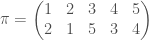 is the permutation that sends 1 to 2, and 2 to 1, 3 to 5 and so on.
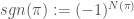 where
where  is the non-identity element in
  (it is easy to see that
  ) and
) and  . Basically
  looks at whether the number of inversions in
  is even or odd. A nice way of visualising permuations is by drawing which elements get sent where. In this way, the permutation
 so that
  and this number is
  . Whether or not this number is even or odd determines the sign. In this case, we see immediately that
  . Deforming a single line can change the number of crossings, but (provided that each crossing is proper and no more than two lines cross at a point) doing so introduces/removes an even number of crossings so the sign is well-defined.
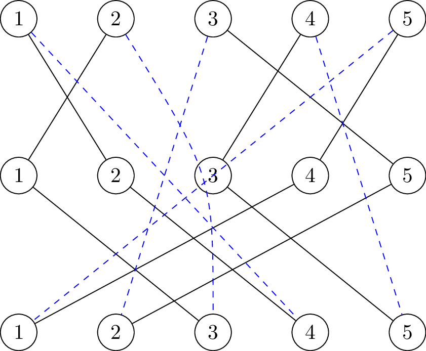
 is a homomorphism. For if we draw the pictures of
  and
and  over each other, we obtain a picture of
  . The total number of crossings is the number of crossings in
  plus the number of crossings in
  the number of crossings in this picture of
  and
and  we have that
  which finishes the proof.
 is an inversion in
 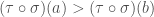 ), then either it is an inversion in
  is an inversion in
  as the alternating group over
  is normal subgroup. For
  it can be shown that
 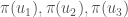 is
is  , where
  . The vertices of both triangles are of course the same, but they are treated as different objects depending on how their vertices are ordered.
 by observing that one line crosses all of the other ones. Knowing that
  disjoint cycles of length
  :
:
 of a group
  is trivial if
  or
or  .
. 